

System Verilog Interview Questions
SystemVerilog is a hardware description and verification language that extends the capabilities of Verilog HDL. It is widely used in the semiconductor industry for the design and verification of digital circuits and systems. If you are preparing for a SystemVerilog interview, you may be asked a variety of questions related to the language, its features, and its applications.
In this blog post, we have compiled a list of commonly asked SystemVerilog interview questions, along with their answers. These questions cover topics such as syntax and semantics, object-oriented programming, testbench development, and verification methodologies. By familiarizing yourself with these questions and their answers, you can prepare yourself to showcase your knowledge of SystemVerilog and increase your chances of landing your desired job in the semiconductor industry.
What is the difference between $display, $write, $monitor, and $strobe in SystemVerilog?
In SystemVerilog, the $display, $write, $monitor, and $strobe tasks are used to display or log messages in a simulation. However, there are some differences in how they are used:
- $display: This task is used to display messages on the console during a simulation. The messages can include text, numbers, and other values. The syntax for $display is similar to that of C's printf function, and it supports format specifiers to control the formatting of the output.
- $write: This task is similar to $display, but it does not automatically add a newline character at the end of the message. This can be useful when you want to print several messages on the same line.
- $monitor: This task is used to monitor signals in a simulation and print out their values when they change. The $monitor task is usually placed inside an initial block or an always block that is triggered by the signals being monitored. The syntax of $monitor is similar to that of $display, but it also includes an argument for the signal being monitored.
- $strobe: This task is used to print out a message at a specific point in time during a simulation. The $strobe task takes a time argument, and the message is printed out when the simulation time reaches that value. This can be useful for debugging or for marking specific points in a simulation.
Overall, these tasks are all useful for debugging and monitoring a simulation, and they can be used in different ways depending on the specific needs of the design.
What is the difference between a packed array and an unpacked array in System Verilog with example?
In System Verilog, an unpacked array is an array that is defined with a fixed size and each element of the array is accessible separately.
Here's an example of an unpacked array in System Verilog:
int myArray[3]; // Unpacked array with size 3
myArray[0] = 10;
myArray[1] = 20;
myArray[2] = 30;
In this example, myArray is an unpacked array of integers with a size of 3. Each element of the array is accessed separately using an index.
A packed array is an array whose elements are grouped together in a single storage unit, and it can be defined with a variable size.
Here's an example of a packed array in System Verilog:
typedef struct packed {
logic [7:0] r;
logic [7:0] g;
logic [7:0] b;
} color_t;
color_t colorArray[] = '{ '{255, 0, 0}, '{0, 255, 0}, '{0, 0, 255} }; // Packed array with 3 elements
In this example, colorArray is a packed array of color_t structs with a variable size. The elements of the array (color_t structs) are packed together in a single storage unit, and each element of the struct (r, g, b) is accessed using the appropriate bit-range.
Note that packed arrays are useful when you need to pack multiple values together, such as in the case of bit-fields or structs. Unpacked arrays are more suited for when you need to access individual elements of the array separately.
Suppose a dynamic array of integers is initialized to values as shown below. Write a code to find all elements greater than 5 in the array using array locator method “ find ”?
int values_arr[] = '{5, 2, 7, 4, 10, 1, 7, 8, 3, 15};
int found_indices[$];
// Find all elements greater than 5 in the array
found_indices = values_arr.find(> 5);
// Print the indices of elements greater than 5
$display("Indices of elements greater than 5:");
foreach (found_indices[i]) begin
$display("%0d", found_indices[i]);
end
This code initializes a dynamic array values_arrto the given values. It then declares an empty dynamic array found_indices to store the indices of elements greater than 5.
The find method is then used to find all elements in values_arr that are greater than 5. The > operator inside the find method specifies the condition for which elements to find.
Finally, the foreach loop is used to print the indices of all elements greater than 5.
How can we use System Verilog constraints to generate a dynamic array with random but unique values with and without unique constraint?
To generate a dynamic array with random but unique values using SystemVerilog constraints, you can follow these steps:
- Determine the size of the array you want to create.
- Create a dynamic array of the determined size using the
randkeyword in the class or struct where you plan to define the constraint.
class MyClass;
rand int myArray[];
endclass
- Define a constraint that ensures unique values in the array using the
uniqueconstraint function. Theuniquefunction takes an argument that specifies the expression to be constrained, and it ensures that all elements in the expression have unique values.
class MyClass;
rand int myArray[];
constraint uniqueValues {
unique(myArray);
}
endclass
- Use the
randomizemethod to generate random values for the array that satisfy the constraint.
class MyClass;
rand int myArray[];
constraint uniqueValues {
unique(myArray);
}
function void generateValues();
randomize(myArray) with {myArray.size() == 10;};
endfunction
endclass
In this example, the generateValues function uses the randomize method to generate 10 random values for the myArray variable that satisfy the uniqueValues constraint. The with clause is used to specify additional constraints on the size of the array, such as a fixed size of 10 elements.
Without using unique constraint, you can still generate incremental values and then do an array shuffle() in post_randomize() method in the class;
constraint c_array_inc_shuffle {
my_array.size == 10 ;// or any size constraint
foreach (myArray[i])
if(i >0) myArray[i] > myArray[i-1];
}
function post_randomize();
myArray.shuffle();
endfunction
Explain the concept of a “ref” and “const ref” argument in SystemVerilog function or task with example?
In SystemVerilog, a "ref" argument is a way to pass an argument to a function or task by reference, meaning that the function or task can modify the value of the argument in the calling scope.
On the other hand, a "const ref" argument is a way to pass an argument by reference, but the function or task is not allowed to modify the value of the argument.
Here's an example to demonstrate the difference between "ref" and "const ref" arguments in a SystemVerilog function:
function void add_numbers_ref(int a, ref int b);
b += a;
endfunction
function void add_numbers_const_ref(int a, const ref int b);
// This line would be a compile error because b is const:
// b += a;
endfunction
module top;
int x = 10;
add_numbers_ref(5, x);
$display("x after add_numbers_ref: %d", x); // Outputs "x after add_numbers_ref: 15"
int y = 20;
add_numbers_const_ref(5, y);
$display("y after add_numbers_const_ref: %d", y); // Outputs "y after add_numbers_const_ref: 20"
endmodule
In this example, the function add_numbers_ref takes two arguments: a, which is passed by value, and b, which is passed by reference using the ref keyword. Inside the function, b is modified to add the value of a. When the function is called in the top module with add_numbers_ref(5, x), x is passed as the second argument and is modified to become 15.
In contrast, the function add_numbers_const_ref takes two arguments: a, which is passed by value, and b, which is passed by const reference using the const ref keywords. Inside the function, b cannot be modified because it is declared as const ref. When the function is called in the top module with add_numbers_const_ref(5, y), y is passed as the second argument, but it is not modified, so its value remains 20.
In summary, ref and const ref arguments in SystemVerilog allow functions and tasks to modify or read arguments in the calling scope, respectively.
Difference between “forever loop” and “for loop” in SystemVerilog?
In SystemVerilog, "forever" and "for" are used to specify the duration of a loop.
The main difference between the two is that "forever" creates an infinite loop that continues until a "break" statement is executed or the simulation is terminated.
If a forever loop is used without any timing controls (like time delay or clock) can result in a zero-delay infinite loop and cause hang in simulation, while "for" create a loop that executes a specified number of times.
Here is an example of a "forever" loop:
forever begin
// Statements to be executed repeatedly
end
In this example, the statements within the "begin" and "end" block will be executed repeatedly until a "break" statement is encountered or the simulation is terminated.
Here is an example of a "for" loop:
for (int i = 0; i < 10; i++) begin
// Statements to be executed repeatedly
end
In this example, the statements within the "begin" and "end" block will be executed 10 times because the loop condition "i < 10" is true for the first 10 iterations of the loop.
So, the main difference between "forever" and "for" is that "forever" creates an infinite loop, while "for" creates a loop that executes a specified number of times.
What is the difference between “case”, “casex” and “casez” in SystemVerilog?
In SystemVerilog, case, casex, and casez are all keywords used for conditional statements, but they differ in how they handle the matching of the case expression to the case items.
casestatement matches the expression with the exact match. The values in thecasestatement must be constants, and the case expression must match one of the constant values specified in the case items.casexstatement performs a case-insensitive match with the "x" wildcard (also known as "don't care") character. It matches the case expression with the case items, allowing "x" in the case items to match with any bit value in the case expression.casezstatement is also a case-insensitive match with "x" wildcard character, but it also matches "z" values in the case items with the "0" or "1" value in the case expression, which means it treats "z" as a wildcard as well.
Here's an example to illustrate the difference between the three:
reg [1:0] x = 2'b11;
case (x)
2'b00: $display("x is 00");
2'b01: $display("x is 01");
2'b10: $display("x is 10");
2'b11: $display("x is 11");
endcase
casex (x)
2'b00: $display("x is 00");
2'b01: $display("x is 01");
2'b1x: $display("x is 10 or 11");
endcase
casez (x)
2'b00: $display("x is 00");
2'b01: $display("x is 01");
2'b1x: $display("x is 10 or 11");
2'bxx: $display("x is unknown");
endcase
In this example, the case statement matches only when the value of x is exactly 2'b00, 2'b01, 2'b10, or 2'b11. The casex statement matches if the value of x is 2'b00, 2'b01, or has a value of 2'b1x (where x can be any value). The casez statement matches if the value of x is 2'b00, 2'b01, or has a value of 2'b1x or 2'bxx.
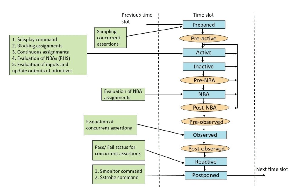
How regions inside a System Verilog simulation semantics works? Explain with Examples
The SystemVerilog scheduling semantics is used to describe the SystemVerilog language element’s behavior and their interaction with each other. This interaction is described with respect to event execution and its scheduling.
The SystemVerilog process concurrently schedules elements such as always, always_comb, always_ff, always_latch, and initial procedural blocks, continuous assignments, asynchronous tasks, and primitives.
Processes are ultimately sensitive to event updates. The terminology of event update describes any change in a variable or net state change. For example, always @(*) is sensitive for all variables or nets used. Any change in variable or net is considered an event update. Another example could be having multiple initial blocks in the code. The evaluation order of these initial blocks can be arbitrary depending on the simulator implementation. Programming Language Interface (PLI) callbacks are used to call a user-defined external routine of a foreign language. Such PLI callbacks are also considered an event that has to be evaluated.
The SystemVerilog language works on the evaluation and execution of such events. So, it becomes important to understand how these events will be evaluated and executed. The events are scheduled in a particular order to render an event execution in a systematic way.
The design takes some time cycles to respond to the driven inputs to produce outputs. The simulator models the actual time for the design description which is commonly known as simulation time. A single time cycle or slot is divided into various regions and that helps out to schedule the events. The simulator executes all the events in the current time slot and then moves to the next time slot. This ensures that the simulation always proceeds forward in time.
What is a modport in an System Verilog Interface?
In SystemVerilog, a modport is a construct that defines a subset of the ports and directions of an interface. A modport allows you to create different views or interfaces of an interface, each with its own set of ports and directions. This can be useful when you have an interface that is used by different modules in different ways, or when you want to limit the access of certain modules to specific parts of an interface.
A modport is defined within an interface and specifies the subset of ports and directions that are available for use. Modports are defined using the modport keyword, followed by a name and a list of ports and directions that are available within the modport.
Here is an example of a modport definition:
interface my_interface(input clk, input rst);
logic [7:0] data_in;
logic [7:0] data_out;
modport master(input data_in, output data_out);
modport slave(output data_in, input data_out);
endinterface
In this example, we have an interface called my_interface with two input ports, clk and rst, and two internal signals, data_in and data_out. We have also defined two modports: master and slave. The master modport has an input data_in port and an output data_out port, while the slave modport has an output data_in port and an input data_out port.
Using these modports, we can create different modules that can connect to the my_interface interface.
For example:
module master_module(my_interface.master interface);
// Implementation of the master module
endmodule
module slave_module(my_interface.slave interface);
// Implementation of the slave module
endmodule
In this example, we have created two modules: master_module and slave_module. The master_module module uses the master modport of the my_interface interface, while the slave_module module uses the slave modport. This allows each module to access a different subset of the interface ports, making it easier to manage and verify the design.
Which of the logical equality operators “==” or “===” are used in case expression conditions for case, casex, and casez?
All of the 3 case statements use “===” logical equality comparison to evaluate condition matches.
What is the difference between byte and logic[7:0] variable in System Verilog?
The main difference between the two is a byte is a signed variable which means it can only be used to count values up to 127 while a logic[7:0] variable can be used for an unsigned 8-bit variable that can count up to 255.
What is the difference between input #1 step sig_1; and input #1ns sig_1; ways of specifying skews in a clocking block?
The difference between the two ways of specifying skews in a clocking block is in the unit of time used to specify the skew.
The first way of specifying the skew is using the "input #1 step" syntax. This means that the signal is sampled one step after the clock edge. The "step" keyword is a relative time unit that is determined by the clock period. So, if the clock period is 1ns, then the "input #1 step" syntax is equivalent to "input #1ns".
The second way of specifying the skew is using the "input #1ns" syntax. This means that the signal is sampled one nanosecond after the clock edge. This is an absolute time unit that is independent of the clock period.
In general, it is recommended to use absolute time units like "ns" or "ps" when specifying skews in a clocking block, as they make the timing requirements more clear and easier to understand. Relative time units like "step" can be more ambiguous and can lead to errors if the clock period is changed. However, using relative time units can be useful in some cases, such as when defining timing requirements for interfaces that are meant to work with different clock frequencies.
Given a dynamic array of size 50, how can the array be re-sized to hold 100 elements while the lower 50 elements are preserved as original in System Verilog?
A dynamic array needs memory initialization using new[] to hold elements. Here is an example of an int my_array that grows from an initial size of 50 elements to 100 elements.
int my_array []; //Dynamic Array Declaration
my_array = new[50]; // Initialize my_array with 50 elements using new[]
// other implementation ....
// Resizes the array to hold 100 elements while the lower 50 elements are preserved as original
my_array = new[100](my_array);
What are pre_randomize() and post_randomize() in System Verilog with example?
In SystemVerilog, pre_randomize() and post_randomize() are two user-defined methods that are called before and after a variable is randomized using the built-in randomization functions.
The pre_randomize() method is called before the variable is randomized, and is used to perform any necessary initialization or setup of the variable. The method is called with the current value of the variable as an argument, and can modify the value before it is randomized.
The post_randomize() method is called after the variable is randomized, and is used to perform any necessary post-processing or validation of the variable. The method is called with the new randomized value of the variable as an argument.
Here's an example of how these methods can be used:
class my_class;
rand int my_variable;
function void pre_randomize(int value);
if (value 100) begin
$display("Value is greater than 100. Changing to 100.");
my_variable = 100;
end
endfunction
endclass
module top;
initial begin
my_class obj = new();
obj.randomize();
$display("my_variable = %0d", obj.my_variable);
end
endmodule
In this example, the pre_randomize() method checks if the initial value of my_variable is less than 0, and changes it to 0 if it is. The post_randomize() method checks if the final randomized value of my_variable is greater than 100, and changes it to 100 if it is.
When the top module is run, it creates an instance of my_class, randomizes the value of my_variable, and prints the final value. The pre_randomize() and post_randomize() methods are called automatically before and after the randomization, respectively.
What is the difference between a union and struct in SystemVerilog with example?
In SystemVerilog, both union and struct are composite data types used for creating custom data types. However, they differ in how they store and access the data.
A struct is a collection of variables of different data types, which are stored in memory as contiguous memory locations. Each variable can be accessed by name, and the variables can be accessed individually or as a whole.
Here is an example of a struct in SystemVerilog:
struct my_struct {
logic [7:0] var1;
bit var2;
int var3;
};
In this example, my_struct is a struct with three variables: var1, var2, and var3. var1 is an 8-bit logic variable, var2 is a single-bit, and var3 is a 32-bit integer. The total memory allocated would be the sum of memory needed for all the data types. Hence in above example, the my_struct struct would take a total memory of 41 bits (8-bit logic + single-bit + 32-bit integer).
These variables are stored in memory as contiguous memory locations and can be accessed by name.
On the other hand, a union is a collection of variables of different data types that share the same memory location. Only one variable in the union can be active at a time, and accessing one variable may affect the value of the others.
Here is an example of a union in SystemVerilog:
union my_union {
logic [7:0] var1;
bit [15:0] var2;
int var3;
};
In this example, my_union is a union with three variables: var1, var2, and var3. However, they share the same memory location. So, if var1 is assigned a value, the value of var2 and var3 may become invalid or undefined, and vice versa. Only one of the variables in the union can be active at a time.
In summary, the main difference between a struct and a union in SystemVerilog is how they store and access the data. A struct stores its variables as contiguous memory locations and each variable can be accessed by name. A union stores its variables at the same memory location and only one variable can be active at a time.
Explain unique constraint in System Verilog with example?
In SystemVerilog, a unique constraint is used to specify that a set of values generated during randomization should be unique. This means that no two values in the set should be equal to each other.
To define a unique constraint in SystemVerilog, you can use the unique keyword followed by the name of the signal or variable that you want to constrain. Here is an example of how to define a unique constraint for a variable my_var:
rand int my_var[$];
constraint my_constraint {
my_var.size() < 10;
unique {my_var};
}
In this example, the my_var variable is an array of integers that can hold up to 10 values. The unique constraint is applied to the entire array, indicating that each value in the array should be unique.
During randomization, the SystemVerilog randomization engine will generate a set of values my_var that satisfy the constraint. Each value in the set will be unique, and no two values will be equal to each other.
Note that if the size of my_var is greater than the number of unique values that can be generated, the randomization engine will return an error. Therefore, it is important to ensure that the size of the variable or signal being constrained is large enough to accommodate the number of unique values required by the constraint.
Which of the array types are good to model really large arrays or a huge memory of 16/32/64KB?
When modeling really large arrays or huge memory sizes of 16/32/64KB, Associative arrays are typically the most suitable option.
Associative arrays, also known as maps or dictionaries, are implemented using a hash table or a binary search tree, which allows for efficient insertion, deletion, and lookup of key-value pairs. However, because the elements are not stored in contiguous memory, accessing an element by index is not as fast and may take O(log n) time.
On the other hand Dynamic arrays, also known as resizable arrays, are implemented as a contiguous block of memory that can be resized as needed. When an element is added to the array and there is no more space available, the array is resized to a larger block of memory, which can be an expensive operation. However, since dynamic arrays use contiguous memory, accessing an element by index is very fast, usually taking O(1) time.
In Summary, Associative arrays are better to model large arrays as memory is allocated only when an entry is written into the array. Dynamic arrays on the other hand need memory to be allocated and initialized before using.
If you want to model a memory array of 16/32/64 KB using a dynamic array, you need to first need allocation and initialization memory of 16/32/64 K entries and use the array for reading/writing. Associative arrays don’t need allocation and initialization of memory upfront and can be allocated and initialized just when an entry of the 16/32/64 K array needs to be referenced. However, associative arrays are also slowest as they internally implement the search for elements in the array using a hash.
Difference between private, public, and protected data members of a SystemVerilog class.
In SystemVerilog, a class is a user-defined type that can contain data members and member functions. The data members of a class can have one of three access modifiers: private, public, or protected.
- Private data members: These data members are only accessible within the class itself. They cannot be accessed or modified by any code outside the class, including derived classes. Private data members are typically used to store internal state or implementation details that should not be exposed to the outside world.
- Public data members: These data members are accessible by any code that can access the class. They can be read or modified by any code that has an instance of the class. Public data members are typically used to provide external access to the state of an object.
- Protected data members: These data members are accessible within the class and its derived classes. They cannot be accessed by any code outside the class hierarchy. Protected data members are typically used to provide access to the state of a class to its derived classes while still keeping it hidden from other code.
In general, it is considered good practice to make data members private and provide public or protected member functions to access or modify them. This helps to encapsulate the implementation details of the class and prevents outside code from directly modifying its state.
What is the difference between new() and new[] in SystemVerilog?
The function new() is the class constructor function in SystemVerilog. It is defined in a class to initialize data members of the class.
The new[] operator is used to allocate memory for a dynamic array. The size of the dynamic array that needs to be created is passed as an argument to the new[].
What is difference between bounded and unbounded mailboxes in System Verilog? Explain with Examples
In SystemVerilog, a mailbox is a communication mechanism that allows data to be exchanged between different threads. Mailboxes can be either bounded or unbounded, which determines the behavior when the mailbox is full.
Bounded mailbox: A bounded mailbox has a fixed size limit, meaning it can only hold a finite number of messages. When the mailbox is full, any attempts to send additional messages will block the sender until there is space available. The receiver can always read messages from the mailbox regardless of whether it is full or not.
mailbox myMailbox = new(4); // create a bounded mailbox with a size limit of 4 messages
// Sender thread
int message = 0;
forever begin
myMailbox.put(message); // put a message in the mailbox
message++;
end
// Receiver thread
int data;
forever begin
myMailbox.get(data); // get a message from the mailbox
$display("Received message: %d", data);
end
In this example, the sender thread will continuously put messages into the mailbox until it is full. When the mailbox is full, the sender thread will block until there is space available. The receiver thread will continuously get messages from the mailbox, regardless of whether it is full or not.
Unbounded mailbox: An unbounded mailbox has no size limit, meaning it can hold an unlimited number of messages. When the mailbox is full, any attempts to send additional messages will not block the sender, and the message will simply be dropped. The receiver can always read messages from the mailbox regardless of whether it is full or not.
Example:
mailbox myMailbox = new(); // create an unbounded mailbox
// Sender thread
int message = 0;
forever begin
myMailbox.put(message); // put a message in the mailbox
message++;
end
// Receiver thread
int data;
forever begin
myMailbox.get(data); // get a message from the mailbox
$display("Received message: %d", data);
end
In this example, the sender thread will continuously put messages into the mailbox, and none of them will be dropped since the mailbox is unbounded. The receiver thread will continuously get messages from the mailbox, regardless of whether it is full or not.
Explain Interfaces in System Verilog with Example
In System Verilog, an interface is a user-defined type that encapsulates a set of signals, their directions, data types, and behavioral functionality.
The main purpose of an interface is to create a standard way of communicating between different modules or sub-modules, and providing a high-level of abstraction.
Interfaces provide a clean separation between different modules in a design, making it easier to manage and verify.
Here is an example of a SystemVerilog interface:
interface bus_interface(
input logic clock,
input logic reset,
output logic [7:0] data_out,
input logic [7:0] data_in
);
logic [15:0] address;
modport master(
output address,
input data_out
);
modport slave(
input address,
output data_in
);
task send_data(output logic [7:0] data);
// Implementation of send_data
endtask
task receive_data(input logic [7:0] data);
// Implementation of receive_data
endtask
endinterface
In this example, we have defined an interface called bus_interface, which has four ports: clock, reset, data_out, and data_in. The interface also has an internal signal called address that is 16 bits wide. The modport keyword is used to create two separate views of the interface: a master view and a slave view.
The master view defines an output address port and an input data_out port. This view can be used by a module that is the master of the bus and needs to write data to a slave device. The slave view defines an input address port and an output data_in port. This view can be used by a module that is the slave of the bus and needs to receive data from the master.
The interface also includes two tasks: send_data and receive_data. These tasks can be used to send or receive data over the bus. The implementation of these tasks would depend on the specific requirements of the design.
Using this interface, we can create different modules that can connect to the bus_interface.
For example:
module bus_master(
bus_interface.master bus
);
// Implementation of the bus master module
endmodule
module bus_slave(
bus_interface.slave bus
);
// Implementation of the bus slave module
endmodule
In this example, we have created two modules: bus_master and bus_slave. The bus_master module has a port that uses the master view of the bus_interface, while the bus_slave module has a port that uses the slave view of the bus_interface. These modules can be connected to the bus using the bus_interface interface, making it easy to reuse the interface across different designs.
What is the difference between a logic, reg and wire in System Verilog?
In SystemVerilog, "logic", "reg", and "wire" are all different data types used to represent variables. Here is a brief overview of the differences between them:
- reg: A "reg" is a variable that can store a binary value (0 or 1) or a multi-bit value or state. A "reg" can be used to model any sequential or combinational logic. A "reg" can be declared as signed or unsigned and can be assigned using blocking or non-blocking assignments. They cannot be driven by a continuous assignment statement.
- wire: A "wire" is a variable used to model combinational logic. A "wire" cannot be assigned using blocking assignments and must always be assigned using continuous assignments and it cannot hold any value if not driven. A "wire" can also be used as a physical wire for a connection between different modules or instances of the same module.
- logic: The "logic" data type was introduced in SystemVerilog to provide a more concise and flexible way to represent variables and it can be used to model both reg as well as the wire. The "logic" data type can be used to represent both single-bit and multi-bit variables, and it supports both signed and unsigned types. The "logic" data type is similar to "reg" in that it can be used to model any combinational or sequential logic, but it is more flexible in terms of the operations that can be performed on it. Logic is a new data type in SystemVerilog that can be used to model both wires and reg. Logic is a 4-state variable and hence can hold 0, 1, x, and z values. If a wire is declared as a wire logic, then it can be used to model multiple drivers and the last assignment will take the value.
In summary, "reg" is used to model sequential or combinational logic and can store binary or multi-bit values, "wire" is used to model combinational logic and can model physical wires to connect two elements, and "logic" is a more flexible data type that can be used to represent both single-bit and multi-bit values and can be used for both combinational and sequential logic.
Explain system tasks and functions in System Verilog? Give some example of system tasks and functions
In SystemVerilog, system tasks and functions are built-in functions and tasks that provide various functionalities and features that are commonly used in hardware design and verification. These built-in system tasks and functions are predefined in the SystemVerilog standard and can be used directly without any need for explicit declaration.
Here are some examples of commonly used system tasks and functions in SystemVerilog:
- $display(): This is a system task that is used to display messages and variables to the standard output. It is primarily used for debugging and diagnostic purposes.
- $random(): This is a system function that is used to generate random numbers during simulation. It is primarily used for testbench development and verification purposes.
- $time(): This is a system function that returns the current simulation time in simulation time units (STUs).
- $fatal(): This is a system task that is used to terminate the simulation immediately and generate an error message.
- $finish(): This is a system task that is used to terminate the simulation gracefully.
These are just a few examples of the many system tasks and functions available in SystemVerilog. The SystemVerilog standard includes a large number of built-in functions and tasks that can be used to implement complex functionalities in hardware design and verification.
Explain the concept of forward declaration of a class in System Verilog with example.
In SystemVerilog, a forward declaration of a class is a way to declare a class without defining its contents.
A forward declaration of a class is typically used when a class needs to refer to another class that has not been fully defined yet. By using a forward declaration, the compiler knows that the class exists, but it does not know anything about its members or methods. This allows the code to compile even if the classes have interdependencies.
Here's an example of how a forward declaration of a class is used:
class ClassA;
// ClassA defined here
endclass
class ClassB;
// Forward declaration of ClassA
extern ClassA my_class_a;
// ClassB defined here, using ClassA
function void do_something();
my_class_a.do_something_else();
endfunction
endclass
In this example, ClassB has a member variable called my_class_a of type ClassA. Since ClassA is defined before ClassB, the forward declaration is not necessary. However, if ClassB were defined before ClassA, the forward declaration would be necessary to avoid a compilation error.
Note that forward declarations are not commonly used in SystemVerilog since the order of class definitions is usually controlled by the user. However, they can be helpful in certain cases where circular dependencies exist or when classes are defined in different files.
What metrics would you use to track the progress of verification project?
Tracking the progress of a verification project is essential to ensure that the project stays on schedule and meets its objectives. Here are some metrics that can be used to track the progress of a verification project:
- Code coverage: Code coverage is a metric that measures the percentage of code that has been exercised during simulation. It can be used to track the progress of test development and ensure that all code paths are being tested.
- Functional coverage: Functional coverage is a metric that measures the percentage of functional requirements that have been verified. It can be used to track the progress of the verification effort and ensure that all functional requirements have been tested.
- Test plan execution status: The test plan execution status tracks the percentage of tests that have been executed and passed. It can be used to track the progress of test execution and identify areas of the design that require further testing.
- Bug tracking: The bug tracking system tracks the number of bugs that have been found and fixed. It can be used to track the progress of bug resolution and ensure that all bugs are being addressed.
- Simulation time: Simulation time is a metric that measures the amount of time required to simulate the design. It can be used to track the progress of the verification effort and identify areas of the design that may require optimization.
- Test bench completeness: Test bench completeness is a metric that measures the percentage of the design that is covered by the test bench. It can be used to track the progress of test bench development and ensure that all parts of the design are being tested.
By monitoring these metrics, the verification team can track the progress of the verification effort, identify areas that require further attention and make adjustments as necessary to ensure that the project stays on schedule and meets its objectives.
In System Verilog How can we merge two events? Explain with example
When one event variable is assigned to another, the two become merged. All processes waiting for the first event to trigger will wait until the second variable is triggered.
Example:
module merged_ev;
event ev_1, ev_2; //declaring event ev_1 and ev_2
initial begin
fork
//process-1, wait for ev_1 to be triggered
begin
wait(ev_1.triggered);
$display($time,"\t Wait for EV_1 is over");
end
//process-2, wait for ev_2to be triggered
begin
wait(ev_2.triggered);
$display($time,"\t Wait for EV_2 is over");
end
#20 ->ev_1; //Triggeres ev_1 at #20
#30 ->ev_2; //Triggeres ev_2 at #30
begin
#10 ev_2 = ev_1; // Assigning events #10
end
join
end
endmodule
Explain clocking block with example and what are the advantages of using clocking blocks inside System Verilog Interface?
A clocking block is a special construct in System Verilog that helps in synchronizing signals between different clock domains. It provides a structured way of defining clock and reset signals, and allows the designer to specify how signals should be sampled or updated at the edges of these signals.
Here is an example of a clocking block:
clocking cb @(posedge clk);
input rst;
output data;
input valid;
default input #1step output #1step;
input @(posedge clk) rst => (data (data <= data+1);
endclocking
In this example, we define a clocking block called "cb" that is sensitive to the positive edge of a clock signal called "clk". It also has an input signal called "rst", an output signal called "data", and an input signal called "valid". The "default" keyword specifies the default timing for inputs and outputs, which is one step delayed from the clock edge. The input and output blocks define the behavior of the signals during the clock edge.
The advantages of using clocking blocks inside the System Verilog Interface are:
- Synchronization: Clocking blocks provide a way to synchronize signals between different clock domains, ensuring that data is sampled and updated correctly.
- Structured design: Clocking blocks allow designers to structure their designs in a more organized and modular way, making them easier to understand and debug.
- Clear intent: Clocking blocks make it clear to other designers what the intent of the signal is, and how it should be used.
- Easy to modify: Since clocking blocks are defined in a separate block, they are easy to modify and update without affecting other parts of the design.
- Increased readability: By using clocking blocks, designers can make their code more readable, which is essential for maintaining a complex design over time.
Identify How many parallel threads does this given code executes?
Given Code:
fork
for (int j=0; j < 15; j++ ) begin
my_task();
end
join
As you can observe that the “for” loop is inside the fork-join, so it executes as a single thread.
How can we disable or enable constraints selectively in a System Verilog class?
In SystemVerilog, you can selectively enable or disable constraints within a class using the constraint_mode() method. This method allows you to set the mode for a constraint block, which can be used to enable or disable a constraint during randomization.
Here's an example of how to enable or disable a constraint in a SystemVerilog class:
class my_class;
rand int x;
rand int y;
constraint my_constraint {
x > y;
}
function void disable_constraint();
constraint_mode(my_constraint, 0);
endfunction
function void enable_constraint();
constraint_mode(my_constraint, 1);
endfunction
endclass
In this example, the my_class class contains two random variables, x and y, and a constraint block named my_constraint. The my_constraint constraint ensures that the value of x is greater than y.
The disable_constraint() method disables the my_constraint constraint by calling constraint_mode(my_constraint, 0). This means that during randomization, the constraint block will be ignored, and values for x and y will be generated without considering the constraint.
The enable_constraint() method enables the my_constraint constraint by calling constraint_mode(my_constraint, 1). This means that during randomization, the constraint block will be taken into account, and values for x and y will be generated such that x is always greater than y.
You can call these methods at any time during the execution of the class to selectively enable or disable the constraint. For example:
my_class obj = new();
obj.randomize(); // the constraint is applied
obj.disable_constraint();
obj.randomize(); // the constraint is ignored
obj.enable_constraint();
obj.randomize(); // the constraint is applied again
In this example, we create an instance of the my_class class, generate random values for x and y using the randomize() method and the constraint are applied because it is enabled by default. We then disable the constraint using the disable_constraint() method, generate random values again, and the constraint is ignored. Finally, we enable the constraint again using the enable_constraint() method, generate random values, and the constraint is applied once again.
In Summary,
//To Disable SV Constraints
.constraint_mode(0); // To disable all constraints
..constraint_mode(0); // To disable specific constraints
//To Enable SV Constraints
.constraint_mode(1); // To Enable all constraints
..constraint_mode(1); // To enable specific constraints
Given a class with following constraints, how can you generate a packet object with address value greater than 500?
Given Class with Constraints:
class my_pkt;
rand bit[15:0] data;
constraint c_data { data inside [0:300];}
endclass
To generate my_pkt an object with a data value greater than 500, you need to modify the constraint c_data to allow values in the desired range. One way to do this is by using the constraint_mode to temporarily disable the existing constraint and then add a new inline constraint to generate data greater than 500.
Here's an example code snippet:
class my_pkt;
rand bit[15:0] data;
constraint c_data { data inside [0:300]; }
endclass
// Example usage:
my_pkt pkt = new();
pkt.c_data.constraint_mode(0);
pkt.randomize with {data > 500;};
$display("my_pkt data = %0d", pkt.data);
Write a system verilog constraint to generate a random value such that it always has 15 bits as 1 and no two bits next to each other should be 1
To generate a random value in System Verilog such that it always has 15 bits as 1 and no two bits next to each other should be 1, you can use the following constraint:
class myClass;
rand bit[64:0] data;
constraint c_data {
$countones(data) ==15;
foreach (data[i])
if(data[i] && i>0)
data[i] != data[i-1];
}
endclass
What is Gate Level Simulation and why is it important in signing off any design?
Gate Level Simulation (GLS) is a type of simulation that verifies the functionality and timing of a digital circuit at the gate level. In GLS, the design is modeled using individual logic gates, and the simulation accounts for delays and timing effects due to the physical properties of the gates, wires, and other components in the circuit.
GLS is important because it allows designers to verify that their digital circuit designs are functioning correctly before fabrication. This is particularly critical in modern chip design, where a single error in a circuit can have catastrophic consequences, such as rendering an entire chip unusable. GLS helps to ensure that the design meets the required specifications and will perform correctly when manufactured.
GLS also helps to identify potential timing issues in the design, such as violations of setup and hold times, which can cause errors in the circuit's output. By simulating the design at the gate level, designers can identify and fix these timing issues before the design is fabricated, saving time and money in the overall design process.
Write System Verilog constraints to generate elements of a dynamic array such that each element of the array is less than 50 and the array size is less than 50.
Here's an example of how you could write System Verilog constraints to generate elements of a dynamic array such that each element of the array is less than 50 and the array size is less than 50:
class my_class;
rand int arr_size;
rand int arr[$];
constraint arr_size inside {1, 49};
constraint arr.size() == arr_size;
constraint foreach (arr[i]) {
arr[i] < 50;
}
endclass
In this example, we define a System Verilog class my_class with two random variables: arr_size, which will be the size of the dynamic array, and arr, which will be the dynamic array itself.
The first constraint arr_size inside {1, 49} limits the array size to be within the range of 1 to 49, ensuring that the array size is less than 50.
The second constraint arr.size() == arr_size sets the size of the dynamic array arr to be equal to arr_size, enforcing that the array size matches the value of arr_size.
Finally, the third constraint foreach (arr[i]) { arr[i] < 50; } iterates over each element of the array arr and enforces that each element is less than 50.
With these constraints in place, we can generate random values for the my_class object and be confident that the resulting dynamic array will have each element less than 50 and the array size less than 50.
Write System Verilog constraints to create a random array such that array size is between 50 and 100 and the values of the array are in descending order?
To create a random array of integers in SystemVerilog such that the array size is between 50 and 100 and the values of the array are in descending order, you can use the following constraints:
rand int dyn_arr [];
constraint array_size {
dyn_arr.size() inside {[50:100]};
}
constraint descending_order {
foreach (dyn_arr[i]) {
if (i > 0) {
dyn_arr[i] < dyn_arr[i-1];
}
}
}
Explanation of constraints:
dyn_arr.size(): This constraint ensures that the size of the arraydyn_arris between 50 and 100, inclusive. Theinsidekeyword is used to specify the range of values.descending_order: This constraint uses aforeachloop to iterate over each element of the arraydyn_arr. Theifstatement inside the loop checks if the current element is greater than the previous element. If it is, the constraint is violated. The<the operator is used to ensure that the values of the array are in descending order.
Hard Constraints Vs Soft Constraints with Examples
Hard Constraints: Hard constraints are rules that must be satisfied by a design. If a hard constraint is violated, the design is considered incorrect or illegal. Hard constraints are typically used to capture design requirements, interface specifications, and timing constraints.
For example, consider the following SystemVerilog code snippet:
class MyClass;
rand int data;
rand bit valid;
constraint data_range { data inside {[0:255]}; }
constraint valid_high { valid == 1; }
endclass
module MyModule;
MyClass obj = new();
always_comb begin
if (obj.valid) begin
// Use obj.data
end
end
endmodule
if a constraint is defined as soft, then the solver will try to satisfy it unless contradicted by another hard constraint or another soft constraint with a higher priority.
Soft constraints are generally used to specify default values and distributions for random variables and can be overridden by specialized constraints.
For example, consider the following SystemVerilog code snippet:
class MyClass;
rand int data;
rand bit valid;
constraint data_range { soft data inside {[0:255]}; }
constraint valid_high { valid == 1; }
endclass
MyClass my_cls = new();
my_cls.randomize() with { data == 300; }
In the above code, if the default constraint did not define as a soft constraint, then the call to randomize would have failed.
Is the given SystemVerilog constraint correct? if yes what will be the output and if no what's wrong with it. Please Explain
class MyClass;
rand bit [7:0] var_1, var_2, var_3;
constraint cls_c { 10 > var_1 > var_2 > var_3; }
endclass
The constraint 10 > var_1 > var_2 > var_3 is invalid in SystemVerilog because it is not well-formed.
The relational operators <, <=, >, >=, ==, and != are used to compare values.
To fix the constraint, it should be rewritten as follows:
constraint cls_c {
var_1 < 10;
var_2 < var_1;
var_3 < var_2;
}
How to override a constraint defined in the base/parent class in the derived/child class?
To override a SystemVerilog constraint defined in the base/parent class in the derived/child class. To do this, you can redefine the constraint in the derived/child class with the same name as the base/parent class constraint.
Here is an example:
class base_class;
rand int x;
constraint c1 { x < 10; }
endclass
class derived_class extends base_class;
constraint c1 { x < 5; } // overriding the constraint defined in the base class
endclass
In this example, the base_class defines a random variable x and a constraint c1 that constrains x to be less than 10. The derived_class extends base_class and overrides the c1 constraint with a new constraint that constrains x to be less than 5.
When you create an object of the derived_class, the c1 constraint defined in the derived_class will be used instead of the c1 constraint defined in the base_class.
When can you say that verification is complete?
Measuring the completeness of verification is an important task to ensure that the design has been thoroughly verified and meets its requirements. However, it can be challenging to determine when verification is complete as there is always a possibility of uncovering new issues or edge cases.
Here are some common approaches to measure the completeness of verification:
- Functional coverage: Functional coverage is a measure of how well the design has been exercised to test its functionality. It is defined by a set of coverage points that capture the functional behavior of the design. The verification team can use functional coverage metrics to determine how well the design has been tested and whether additional testing is necessary.
- Code coverage: Code coverage is a measure of how much of the design code has been executed during simulation. It can be used to track the completeness of the test suite and ensure that all code paths have been tested.
- Bug count: The number of bugs found during the verification process is another measure of completeness. The verification team can set a threshold for the maximum number of bugs allowed, and once that threshold is reached, additional testing can be performed to ensure that all issues have been addressed.
- Simulation time: Simulation time is a measure of how much time has been spent simulating the design. The verification team can use simulation time as an indicator of completeness and identify areas of the design that require optimization or additional testing.
- Requirements coverage: Requirements coverage is a measure of how well the design requirements have been verified. It can be used to track the completeness of the verification effort and ensure that all requirements have been tested.
In general, the completeness of verification is determined based on a combination of these factors, and it is up to the verification team to determine when they have achieved sufficient coverage to declare verification complete. Typically, the decision to declare verification complete is based on a combination of coverage metrics, budget constraints, and risk tolerance. Once verification is complete, the design can move on to the next stage of the development process, such as synthesis, place, and route.
I tried to reframe questions and answers from Semiconductor Industry experts and all Credit goes to the original author’s work is a crucial part of ethical writing and research who’s nonother than Mr. Robin Garg and Mr. Ramdas Mozhikunnath‘s knowledge and exposure to the semiconductor industry over the last so many years. I really like the way they shared their knowledge with the engineers who are in VLSI Domain.
Books to refer to as a Verification Engineer to learn System Verilog in more detail:
- Writing Testbenches using SystemVerilog by Janick Bergeron – https://amzn.to/3ndnXop
- SystemVerilog for Verification by Chris Spear – https://amzn.to/3zSzG3k
- Verilog and System Verilog Gotchas by Stuart Southerland – https://amzn.to/3bi0ShE
- SystemVerilog Assertions Handbook: for Formal and Dynamic Verification By Ben Cohen, Srinivasan Venkataramanan, Ajeetha Kumari – https://amzn.to/3n9p1tu
- Principles of Functional Verification by Andreas Meyer – https://amzn.to/3OzNh3Y
- System Verilog Assertions and Functional Coverage – Guide to Language Methodology and Applications by Ashok B Mehta – https://amzn.to/39JRyTA
- A Practical Guide for SystemVerilog Assertions by Srikanth Vijayaraghvan, Meyappan Ramanathan – https://amzn.to/3zTTeV2
- Introduction to SystemVerilog by Ashok B Mehta – https://amzn.to/3zQCRZl


Maybe stupid, regarding the definition of a wire
Wire a;
Assign a=en? In : a; // can be used to model a hold on a value when en==0
It’s a different way to use but it doesn’t mean wire holds a value just like reg.
hey, good job
Thank you Alin Mocanu 🙂 Please share with your friends so it will reach to everyone who seeks knowledge 🙂
Excellent post. I was checking continuously this blog and I am impressed!
Extremely usefful information. I care for such innformation a lot.
I was looking for this certain information for a very long
time.Thahk you and goood luck.
Thank you 🙂 Please share this with your friends and network 🙂
I have a question on code coverage.
there is a 4bit variable lets say [0:15]a, 0 to 11 values of code should get 100% coverage and 12 to 15 values must be excluded. How can we write this code coverage?
Hi Sreeja,
Are you sure you want to write code coverage? Can Verification Engineer write code coverage?
Thank you
Here a is not storing any value, its being driven continously
29. Given a 32 bit address field as a class member, write a constraint to generate a random value such that it always has 10 bits as 1 and no two bits next to each other should be 1
class packet;
rand bit[31:0] addr;
constraint c_addr {
$countones(addr) ==10;
foreach (addr[i])
if(addr[i] && i>0)
addr[i] != addr[i-1];
}
endclass
Great job!.
I don’t think this code works for the given question because foreach will be looking for a two dimensional array. Please correct me if I’m wrong.
It would be great if you post more problem-solving questions for constraints
Hi Kavya,
Thanks, for visiting the blog post. Can you please help me to know why it will look for a 2-dimensional array here and did you try this example in your code?
Excellent collection & explaination of all topics !! just Great.
Thanks Vicky 🙂